

① L2 Nearest neighbors in feature/pixel space
② Dimensionality Reduction 4096 차원 -> 2 차원 : PCA, t-SNE, UMAP
Maximally Activating Patches
Run many images through the network -> record values of chosen channel -> Visualize image pathes that correspond to maximal activations
Which Pixels Matter? Saliency via Occlusion
Make part of the image before feeding to CNN, check how much predicted probabilities change

* computational expensive
Which Pixels Matter? Saliency via Backprop
Compute gradient of (unnormalized) class score with respect to image pixels, take absolute value and max over RGB channels. - 기울기 계산

+ Saliency Maps : Segmentation without Supervision (배경없이 물체만 추출해내기)

Intermediate Features via (guided) backprop
Pick a single intermediate neuron, and Compute gradient of neuron value with respect to image pixels.

Images come out nicer if you only backprop positive gradients through each ReLU (guided backprop)

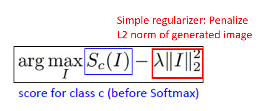
Visualizing CNN Feature: Gradient Ascent
(Guided) backprop은 neuron이 반응하는 이미지의 부분을 찾는 것이고, Gradient ascent는 neuron을 가장 크게 활성화시키는 가짜 이미지를 생성하는 것이다.

Repeat:
1. Initialize image to zeros
2. Forward image to compute current scores
3. Backprop to get gradient of neuron value with respect to image pixels
4. Make a small update to the image
Better regularization : Penalize L2 norm of image; also during optimization periodically
① Gaussian blur image
② Clip pixels with small values to 0
③ Clip pixels with small gradients to 0
+ Adding "multi-faceted" visualization gives even nicer results
(+ more careful regularization, center-bias)

Adverarial Examples
1. Start from an arbitrary image
2. Pick an arbitrary category
3. Modify the image (via gradient ascent) to maximize the class score
4. Stop when the network is fooled

Feature Inversion
Given a CNN feature vector for an image, find a new image that:
- Matches the given feature vector
- "looks natural" (image prior regularization)

ex) reconstructing from different layers of VGG-16

DeepDream : Amplify Existing Features
Rather than synthesizing an image to maximize a specific neuron,
instead try to amplify the neuron activations at some layer in the network


Choose an image and a layer in a CNN; repeat:
1. Forward: compute activations at chosen layer
2. Set gradient of chosen layer equal to its activation
3. Backward: Compute gradient on image
4. Update image
lower layer -> higher layer : 좀더 패턴이 보이고 구체화 됨.
Texture Synthesis
Given a sample patch of some texture, can we generate a bigger image of the same texture?

Nearest Neighbor
Generate pixels one at a time in scanline order;
form neighborhood of already generated pixels and copy nearest neighbor from input

Gram Matrix
- Each layer of CNN gives C x H x W tensor of features; H x W grid of C-dimensional vectors.
- Outer product of two C-dimensional vectors gives C x C matrix of elementwise products.
- Average over all HW pairs gives Gram Matrix of shape C x C giving unnormalized covariance
- Efficient to compute; reshape features from C x H x W to F = C x HW

Neural Texture Synthesis
Reconstructing texture from higher layers recovers larger features from the input texture.

Texture synthesis ~ Feature reconstruction
Neural Style Transfer
(-> Using instance Normalization)


+ Mix style from multiple images by taking a weighted average of Gram matrices
Problem : Style transfer requires many forward/backward passes through VGG; very slow!
Solution : Train another neural network to perform style transfer for us!
(1) Train a feedforward network for each style
(2) Use pretrained CNN to compute same losses as before
(3) After training, stylize images using a single forward pass
+ One network, Many Styles
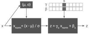
Use the same network for multiple styles using conditional instance normalization:
learn separate scale and shift parameters per style.
Summary
Many methods for understanding CNN representations
Activations: Nearest neighborsm Dimensionality reduction, maximal patchesm occlusion, CAM
Gradients: Grad-CAM, Saliency maps, class visualization, fooling images, feature inversion
Fun: DeepDream, Style Transfer
'Open Lecture Review > Deep Learning for Computer Vision' 카테고리의 다른 글
| Lecture 20: Generative Models 2 (0) | 2022.02.27 |
|---|---|
| Lecture 19: Generative Models 1 (0) | 2022.02.18 |
| Lecture 13: Attention 1 (0) | 2022.02.18 |
| Lec12_Recurrent Neural Networks (0) | 2022.02.14 |
| Lecture 11_Training Neural Networks 2 (0) | 2022.02.13 |


